Using POPCON to Compute Fluxes and Inductances Over Ramp-Up and Flattop
By I. Savona
This notebook demonstrates how to calculate an estimate of the flux consumption over the ramp-up for time-independent POPCONs.
[1]:
%reload_ext autoreload
%autoreload 2

import xarray as xr
import numpy as np
import matplotlib.pyplot as plt
from pathlib import Path

import cfspopcon
from cfspopcon.unit_handling import ureg, Quantity, magnitude_in_units
from cfspopcon.algorithm_class import Algorithm, CompositeAlgorithm
from cfspopcon import named_options

# Change to the top-level directory. Required to find radas_dir in its default location.
%cd {Path(cfspopcon.__file__).parents[1]}
# As a sanity check, print out the current working directory
print(f"Running in {Path('').absolute()}")
/Users/tbody/Projects/cfspopcon
Running in /Users/tbody/Projects/cfspopcon
Defining a Machine object to store info about tokamaks from all over the world!
Here, we use a few (outdated) SPARC designs as well as a few other tokamaks.
N.b. these SPARC designs and other devices are to demonstrate the flux consumption functionality, and should not be assumed to be correct or relevant
[2]:
class Machine:
    def __init__(self, B0, R0, a, delta, kappa, Ip):
        self.magnetic_field_on_axis = Quantity(B0, ureg.T)
        self.major_radius           = Quantity(R0, ureg.m)
        self.minor_radius           = Quantity(a, ureg.m)
        self.triangularity_psi95    = Quantity(delta, ureg.dimensionless)
        self.inverse_aspect_ratio   = a / R0
        self.areal_elongation       = Quantity(kappa, ureg.dimensionless)
        self.plasma_current         = Quantity(Ip, ureg.MA)

machine = dict()
machine["SPARCV1D"] = Machine(B0=12.3, R0=1.845, a=0.565, delta=0.55,  kappa=1.7,  Ip=8.7)
machine["SPARCV0D"] = Machine(B0=12,   R0=1.65,  a=0.56,  delta=0.32,  kappa=1.8,  Ip=7.5)
machine["JT60-SA"]  = Machine(B0=2.72, R0=3.01,  a=1.14,  delta=0.57,  kappa=1.85, Ip=5.5)
machine["DIII-D"]   = Machine(B0=2.6,  R0=1.66,  a=0.67,  delta=0.45,  kappa=1.76, Ip=1.2)
machine["ITER"]     = Machine(B0=5.3,  R0=6.2,   a=2.0,   delta=0.33,  kappa=1.70, Ip=15.0)
machine["KSTAR"]    = Machine(B0=3.5,  R0=1.8,   a=0.5,   delta=0.8,   kappa=2.0,  Ip=2.0)
machine["FIRE"]     = Machine(B0=10.0, R0=2.0,   a=0.525, delta=0.4,   kappa=1.8,  Ip=6.5)
machine["ASDEX-U"]  = Machine(B0=2.5,  R0=1.65,  a=0.5,   delta=0.4,   kappa=1.8,  Ip=1.4)
machine["JET"]      = Machine(B0=3.6,  R0=2.96,  a=1.25,  delta=0.45,  kappa=1.68, Ip=5)
machine["EAST"]     = Machine(B0=3.5,  R0=1.85,  a=0.45,  delta=0.8,   kappa=2.0,  Ip=1.0)
machine["ALC-CMOD"] = Machine(B0=9.5,  R0=0.64,  a=0.21,  delta=0.5,   kappa=1.8,  Ip=2.02)
Update dataset and calculate inductances and fluxes during flattop
We want to run the flux consumption algorithms. However, these rely on a number of other algorithms. We could perform these calculations one-by-one, but it’s easier to build a single CompositeAlgorithm which we can run in a single step.
[3]:
algorithms = [
    "calc_minor_radius_from_inverse_aspect_ratio",
    "calc_plasma_poloidal_circumference",
    "calc_plasma_volume",
    "calc_elongation_at_psi95_from_areal_elongation",
    "calc_average_ion_temp_from_temperature_ratio",
    "calc_f_shaping_for_qstar",
    "calc_q_star_from_plasma_current",
    "calc_beta_toroidal",
    "calc_beta_poloidal",
    "calc_effective_collisionality",
    "calc_ion_density_peaking",
    "calc_electron_density_peaking",
    "calc_bootstrap_fraction",
    "calc_inductive_plasma_current",
    "calc_Spitzer_loop_resistivity",
    "calc_resistivity_trapped_enhancement",
    "calc_neoclassical_loop_resistivity",
    "calc_loop_voltage",
    "calc_cylindrical_edge_safety_factor",
    "calc_internal_inductivity",
    "calc_internal_inductance_for_noncylindrical",
    "calc_external_inductance",
    "calc_vertical_field_mutual_inductance",
    "calc_invmu_0_dLedR",
    "calc_vertical_magnetic_field",
    "calc_internal_flux",
    "calc_external_flux",
    "calc_resistive_flux",
    "calc_poloidal_field_flux",
    "calc_flux_needed_from_solenoid_over_rampup",
    "calc_max_flattop_duration",
    "calc_breakdown_flux_consumption",
]

algs = []

for key in algorithms:
    algs.append(Algorithm.get_algorithm(key))

calc_flux_and_inductance_dependencies = CompositeAlgorithm(algs)
The CompositeAlgorithm can be run in a single step, returning an xr.Dataset of results.
N.b. We have used a custom internal inductivity because the cylindrical l_i was seen to differ as much as 46% as compared to the l_i calculated by the TSC. Because estimations of l_i tend not to be reliable (as a true calculation relies on equilibrium reconstruction) an l_i from simulation is recommended.
[4]:
dataset = calc_flux_and_inductance_dependencies.run(
    major_radius = machine["SPARCV1D"].major_radius,
    areal_elongation = machine["SPARCV1D"].areal_elongation,
    triangularity_psi95 = machine["SPARCV1D"].triangularity_psi95,
    magnetic_field_on_axis = machine["SPARCV1D"].magnetic_field_on_axis,
    plasma_current = machine["SPARCV1D"].plasma_current,
    inverse_aspect_ratio = machine["SPARCV1D"].inverse_aspect_ratio,
    elongation_ratio_areal_to_psi95 = 1.025,
    average_electron_density = 2.5 * ureg.n20,
    average_electron_temp = 9.0 * ureg.keV,
    ion_to_electron_temp_ratio = 1.0,
    surface_inductance_coefficients = named_options.SurfaceInductanceCoeffs.Barr,
    total_flux_available_from_CS = 35.0 * ureg.Wb,
    ejima_coefficient = 0.6,
    z_effective = 1.5,
    electron_density_peaking_offset = -0.1,
    ion_density_peaking_offset = -0.2,
    temperature_peaking = 2.5,
    dilution = 0.85,
)

dataset["max_flux_for_flattop"] = (
    dataset["total_flux_available_from_CS"] - dataset["flux_needed_from_CS_over_rampup"]
)

dataset["total_flux_consumed_over_rampup"] = (
    dataset["internal_flux"] + dataset["external_flux"] + dataset["resistive_flux"]
)
dataset["rule_of_thumb_flux_consumed_over_rampup"] = (
    magnitude_in_units(2.0 * dataset["major_radius"] * dataset["plasma_current"], ureg.m * ureg.MA) * ureg.Wb
)
Let’s print out the quantities computed by these algorithms.
[5]:
for variable in [
    "beta_poloidal",
    "internal_inductivity",
    "internal_inductance",
    "external_inductance",
    "vertical_field_mutual_inductance",
    "vertical_magnetic_field",
    "areal_elongation",
    "major_radius",
    "inverse_aspect_ratio",
    "plasma_current",
    "internal_flux",
    "external_flux",
    "resistive_flux",
    "loop_voltage",
    "max_flattop_duration",
    "magnetic_field_on_axis",
    "poloidal_field_flux",
    "total_flux_consumed_over_rampup",
    "rule_of_thumb_flux_consumed_over_rampup",
    "max_flux_for_flattop",
]:
    print(f"{variable:40} | {dataset[variable].item()}")
beta_poloidal                            | 0.19105621337737821 dimensionless
internal_inductivity                     | 1.2262130634274102 dimensionless
internal_inductance                      | 1.2014505500199678e-06 henry
external_inductance                      | 2.734033460324752e-06 henry
vertical_field_mutual_inductance         | 1.0290112526513495 dimensionless
vertical_magnetic_field                  | 1.169420269348009 tesla
areal_elongation                         | 1.7 dimensionless
major_radius                             | 1.845 meter
inverse_aspect_ratio                     | 0.3062330623306233
plasma_current                           | 8.7 megaampere
internal_flux                            | 10.452619785173718 weber
external_flux                            | 23.78609110482534 weber
resistive_flux                           | 12.102545881620241 weber
loop_voltage                             | 0.18016883201106373 volt
max_flattop_duration                     | 8.477626485735943 second
magnetic_field_on_axis                   | 12.3 tesla
poloidal_field_flux                      | 12.868660833780403 weber
total_flux_consumed_over_rampup          | 46.3412567716193 weber
rule_of_thumb_flux_consumed_over_rampup  | 32.102999999999994 weber
max_flux_for_flattop                     | 1.5274040621611036 weber
The assumption here is that at t=0 the flux-consuming terms are 0 webers and so the flux value at flattop is a reasonable estimate on the change in flux over the ramp-up.
The poloidal flux is included in the estimate for total flux since this function gives the instantaneous flux contribution from the poloidal field coils to the LCFS of the plasma via the vertical field to maintain the toroidal force balance.
We can now do the same calculation of flux consumed over the ramp-up for various machines and compare the method used above with a Rule of Thumb (ROT) and a method employed by Sugihara.
[6]:
from scipy import constants

def calc_flux_rampup_Sugihara(kappa:float, R:float, a:float, Ip:float) -> float:
    R = R.item().magnitude
    kappa = kappa.item().magnitude
    a = a.item().magnitude
    Ip = Ip.item().magnitude
    A = R/a
    flux_Ind = constants.mu_0*A*a*(np.log(8*A)-1.6)*(Ip*1e6)
    flux_Res = 3.78e-6*(kappa**(0.2))*((R)/((a)**0.8))*((Ip*1e6)**0.8)
    return flux_Res + flux_Ind

def calc_flux_rampup_ROT(R:float, Ip:float) -> float:
    return (2 * R.item().magnitude * Ip.item().magnitude)

def reltol (other, poynt):
    return '{:g}'.format(float('{:.{p}g}'.format(100 * np.abs(other-poynt)/other, p=3)))
With our Machine objects we can construct a DataArray with the various methods for calculating the flux over the ramp up. Note that the Sugihara method does not explicitly take into account the flux contribution from the vertical field created by the PFCs.
[7]:
flux_methods_over_machines = xr.DataArray(
    dims=["machine", "flux_method"],
    coords=dict(
        machine=["ALC-CMOD", "ASDEX-U", "DIII-D", "EAST", "FIRE", "ITER", "JET", "JT60-SA", "KSTAR", "SPARCV1D", "SPARCV0D"],
        flux_method=["Hirsh&MitTaka13", "Hirsh&Barr", "Hirsh&Jean", "Hirsh&MFEF", "Barr&Barr", "ROT", "Sugihara"],
    ),
)
PF_flux_over_machines = flux_methods_over_machines.copy(deep=True)
[8]:
algorithms = [
    "calc_plasma_volume",
    "calc_plasma_poloidal_circumference",
    "calc_internal_inductance_for_noncylindrical",
    "calc_external_inductance",
    "calc_vertical_field_mutual_inductance",
    "calc_invmu_0_dLedR",
    "calc_vertical_magnetic_field",
    "calc_internal_flux",
    "calc_external_flux",
    "calc_resistive_flux",
    "calc_poloidal_field_flux",
    "calc_flux_needed_from_solenoid_over_rampup",
]

algs = []

for key in algorithms:
    algs.append(Algorithm.get_algorithm(key))

calc_flux_and_inductance_dependencies_over_machines = CompositeAlgorithm(algs)
We can then make other assumptions about flattop parameters across all machines and make a dictionary for the different calculation methods…
[9]:
# dictionary of the various flux calculation methods to make iterating easier
external_flux_method_dict = {
    "Hirsh&MitTaka13": (named_options.SurfaceInductanceCoeffs.Hirshman, named_options.VertMagneticFieldEq.Mit_and_Taka_Eq13),
    "Hirsh&Barr": (named_options.SurfaceInductanceCoeffs.Hirshman, named_options.VertMagneticFieldEq.Barr),
    "Hirsh&Jean": (named_options.SurfaceInductanceCoeffs.Hirshman, named_options.VertMagneticFieldEq.Jean),
    "Hirsh&MFEF": (named_options.SurfaceInductanceCoeffs.Hirshman, named_options.VertMagneticFieldEq.MagneticFusionEnergyFormulary),
    "Barr&Barr": (named_options.SurfaceInductanceCoeffs.Barr, named_options.VertMagneticFieldEq.Barr),
    "ROT": (named_options.SurfaceInductanceCoeffs.Hirshman, named_options.VertMagneticFieldEq.MagneticFusionEnergyFormulary),
    "Sugihara": (named_options.SurfaceInductanceCoeffs.Barr, named_options.VertMagneticFieldEq.Barr),
}
Before we see the results over all machines, it is first nice to see how different flux calculation methods for various components of flux comare for the SPARCV1D machine parameters…
[10]:
import warnings
warnings.filterwarnings('ignore') # ignore unit strip warning happening with Sugihara and ROT functions
###***RUN CALCULATIONS***###
for machine_name in machine:
    for external_flux_method in external_flux_method_dict:
        if external_flux_method != "ROT" and external_flux_method != "Sugihara":
            dataset = calc_flux_and_inductance_dependencies_over_machines.run(
            magnetic_field_on_axis = machine[machine_name].magnetic_field_on_axis,
            major_radius = machine[machine_name].major_radius,
            minor_radius = machine[machine_name].minor_radius,
            triangularity_psi95 = machine[machine_name].triangularity_psi95,
            areal_elongation = machine[machine_name].areal_elongation,
            inverse_aspect_ratio = machine[machine_name].inverse_aspect_ratio,
            plasma_current = machine[machine_name].plasma_current,
            surface_inductance_coefficients = external_flux_method_dict[external_flux_method][0],
            vertical_magnetic_field_equation = external_flux_method_dict[external_flux_method][1],
            beta_poloidal = 0.1 ,
            loop_voltage = 0.5 * ureg.volts,  # N/A for this calc since not considering flattop
            elongation_ratio_sep_to_areal = 1,
            triangularity_ratio_sep_to_psi95 = 1,
            ejima_coefficient = 0.6,
            internal_inductivity = 0.91,
            total_flux_available_from_CS = 0 * ureg.weber  # N/A for these calcs
            )
            # STORE VALUES
            PF_flux_over_machines.loc[dict(machine=machine_name, flux_method=external_flux_method)] = dataset["poloidal_field_flux"]
            if machine_name == "SPARCV1D":
                SPARCV1D_external_flux = dataset.get("external_flux").item()
                SPARCV1D_internal_flux = dataset.get("internal_flux").item()
                SPARCV1D_resistive_flux = dataset.get("resistive_flux").item()
                SPARCV1D_PF_flux = dataset.get("poloidal_field_flux").item()
                print(
                    external_flux_method,
                    ": ",
                    "SPARCV1D_resistive_flux ",
                    SPARCV1D_resistive_flux,
                    "SPARCV1D_external_flux ",
                    SPARCV1D_external_flux,
                    "SPARCV1D_internal_flux ",
                    SPARCV1D_internal_flux,
                    "SPARCV1D_PF_flux ",
                    SPARCV1D_PF_flux,
                    "flux_needed_from_CS_for_ramp",
                    dataset.get("flux_needed_from_CS_over_rampup").item(),
                )
            flux_methods_over_machines.loc[dict(machine=machine_name, flux_method=external_flux_method)] = dataset[
                "flux_needed_from_CS_over_rampup"
            ]
        elif external_flux_method == "ROT":
            ROT_flux = calc_flux_rampup_ROT(dataset.get("major_radius"), dataset.get("plasma_current"))
            flux_methods_over_machines.loc[dict(machine=machine_name, flux_method=external_flux_method)] = (
                ROT_flux * ureg.weber
            )
        elif external_flux_method == "Sugihara":
            Sugihara_flux = calc_flux_rampup_Sugihara(
                dataset.get("areal_elongation"), dataset.get("major_radius"), dataset.get("minor_radius"), dataset.get("plasma_current")
            )
            flux_methods_over_machines.loc[dict(machine=machine_name, flux_method=external_flux_method)] = Sugihara_flux * ureg.weber
Hirsh&MitTaka13 :  SPARCV1D_resistive_flux  12.102545881620241 weber SPARCV1D_external_flux  18.5199760409476 weber SPARCV1D_internal_flux  7.757121733739522 weber SPARCV1D_PF_flux  7.526116577635606 weber flux_needed_from_CS_for_ramp 30.85352707867176 weber
Hirsh&Barr :  SPARCV1D_resistive_flux  12.102545881620241 weber SPARCV1D_external_flux  18.5199760409476 weber SPARCV1D_internal_flux  7.757121733739522 weber SPARCV1D_PF_flux  7.495799244364226 weber flux_needed_from_CS_for_ramp 30.88384441194314 weber
Hirsh&Jean :  SPARCV1D_resistive_flux  12.102545881620241 weber SPARCV1D_external_flux  18.5199760409476 weber SPARCV1D_internal_flux  7.757121733739522 weber SPARCV1D_PF_flux  7.781319888717262 weber flux_needed_from_CS_for_ramp 30.598323767590102 weber
Hirsh&MFEF :  SPARCV1D_resistive_flux  12.102545881620241 weber SPARCV1D_external_flux  18.5199760409476 weber SPARCV1D_internal_flux  7.757121733739522 weber SPARCV1D_PF_flux  8.787145773802301 weber flux_needed_from_CS_for_ramp 29.592497882505064 weber
Barr&Barr :  SPARCV1D_resistive_flux  12.102545881620241 weber SPARCV1D_external_flux  23.677972398615267 weber SPARCV1D_internal_flux  7.757121733739522 weber SPARCV1D_PF_flux  11.595798286355278 weber flux_needed_from_CS_for_ramp 31.94184172761976 weber
Now we can visualize the different calculation methods for the flux necessary from the central solenoid over a purely ohmic rampup across various machines. In other words: how much flux is needed from the CS over a purely ohmic rampup given certain flattop conditions?
[11]:
import pandas as pd

###***Scaling other machines to create a clearer bar plot***###
machine_name = flux_methods_over_machines.coords['machine'].values
scaled_machine_name = list(machine_name.copy())  # Convert to list for easier manipulation
print(scaled_machine_name)

scaling_factor_ITER =  flux_methods_over_machines.loc[dict(machine="SPARCV1D")] / flux_methods_over_machines.loc[dict(machine="ITER")]
scaling_factor_CMOD =  flux_methods_over_machines.loc[dict(machine="SPARCV1D")] / flux_methods_over_machines.loc[dict(machine="ALC-CMOD")]
scaling_factor_AUG =   flux_methods_over_machines.loc[dict(machine="SPARCV1D")] / flux_methods_over_machines.loc[dict(machine="ASDEX-U")]
scaling_factor_DIIID = flux_methods_over_machines.loc[dict(machine="SPARCV1D")] / flux_methods_over_machines.loc[dict(machine="DIII-D")]
scaling_factor_EAST =  flux_methods_over_machines.loc[dict(machine="SPARCV1D")] / flux_methods_over_machines.loc[dict(machine="EAST")]
scaling_factor_FIRE =  flux_methods_over_machines.loc[dict(machine="SPARCV1D")] / flux_methods_over_machines.loc[dict(machine="FIRE")]
scaling_factor_KSTAR = flux_methods_over_machines.loc[dict(machine="SPARCV1D")] / flux_methods_over_machines.loc[dict(machine="KSTAR")]

scaled_machine_name[5] = str("{:.2g}".format(scaling_factor_ITER.mean().values)) + "*" + scaled_machine_name[5]
scaled_machine_name[0] = str("{:.2g}".format(scaling_factor_CMOD.mean().values)) + "*" + scaled_machine_name[0]
scaled_machine_name[1] = str("{:.2g}".format(scaling_factor_AUG.mean().values)) + "*" + scaled_machine_name[1]
scaled_machine_name[2] = str("{:.2g}".format(scaling_factor_DIIID.mean().values)) + "*" + scaled_machine_name[2]
scaled_machine_name[3] = str("{:.2g}".format(scaling_factor_EAST.mean().values)) + "*" + scaled_machine_name[3]
scaled_machine_name[4] = str("{:.2g}".format(scaling_factor_FIRE.mean().values)) + "*" + scaled_machine_name[4]
scaled_machine_name[8] = str("{:.2g}".format(scaling_factor_KSTAR.mean().values)) + "*" + scaled_machine_name[8]

scaled_machine_name = np.array(scaled_machine_name)

flux_methods_over_machines.loc[dict(machine="ITER")] = scaling_factor_ITER.mean() * flux_methods_over_machines.loc[dict(machine="ITER")]
flux_methods_over_machines.loc[dict(machine="ALC-CMOD")] = scaling_factor_CMOD.mean() * flux_methods_over_machines.loc[dict(machine="ALC-CMOD")]
flux_methods_over_machines.loc[dict(machine="ASDEX-U")] = scaling_factor_AUG.mean() * flux_methods_over_machines.loc[dict(machine="ASDEX-U")]
flux_methods_over_machines.loc[dict(machine="DIII-D")] = scaling_factor_DIIID.mean() * flux_methods_over_machines.loc[dict(machine="DIII-D")]
flux_methods_over_machines.loc[dict(machine="EAST")] = scaling_factor_EAST.mean() * flux_methods_over_machines.loc[dict(machine="EAST")]
flux_methods_over_machines.loc[dict(machine="FIRE")] = scaling_factor_FIRE.mean() * flux_methods_over_machines.loc[dict(machine="FIRE")]
flux_methods_over_machines.loc[dict(machine="KSTAR")] = scaling_factor_KSTAR.mean() * flux_methods_over_machines.loc[dict(machine="KSTAR")]
flux_methods_over_machines = flux_methods_over_machines.assign_coords(machine=scaled_machine_name)


###***PLOTTING_needed_CS_flux_over_rampup***###
df = pd.DataFrame(
    {
        "Hirsh&MitTaka13": flux_methods_over_machines.sel(machine=scaled_machine_name, flux_method="Hirsh&MitTaka13"),
        "Hirsh&Barr": flux_methods_over_machines.sel(machine=scaled_machine_name, flux_method="Hirsh&Barr"),
        "Hirsh&Jean": flux_methods_over_machines.sel(machine=scaled_machine_name, flux_method="Hirsh&Jean"),
        "Hirsh&MFEF": flux_methods_over_machines.sel(machine=scaled_machine_name, flux_method="Hirsh&MFEF"),
        "Barr&Barr": flux_methods_over_machines.sel(machine=scaled_machine_name, flux_method="Barr&Barr"),
        "ROT": flux_methods_over_machines.sel(machine=scaled_machine_name, flux_method="ROT"),
        "Sugihara": flux_methods_over_machines.sel(machine=scaled_machine_name, flux_method="Sugihara"),
    },
    index=scaled_machine_name,
)

ax = df.plot.bar(
    figsize=(15, 5),
    rot=0,
    width=0.95,
    color={
        "Hirsh&MitTaka13": "xkcd:grass green",
        "Hirsh&Barr": "xkcd:scarlet",
        "Hirsh&Jean": "xkcd:ocean blue",
        "Hirsh&MFEF": "xkcd:pumpkin",
        "Barr&Barr": "xkcd:purple",
        "ROT": "xkcd:dark yellow",
        "Sugihara": "xkcd:brown",
    },
)
for p in ax.patches:
    label = "{:.2g}".format(p.get_height())  # Round to two decimal places
    ax.annotate(
        str(label),
        (p.get_x() + p.get_width() / 2.0, p.get_height()),
        ha="center",
        va="center",
        fontsize=7,
        xytext=(0, 5),
        textcoords="offset points",
        color="black",
        weight="bold",
    )
ax.set_ylabel("Flux from Central Solenoid [Weber]")
ax.set_title("Necessary Flux from the Central Solenoid for a Purely Ohmic Rampup")
ax.legend(loc="lower left")

ax.set_xticklabels(scaled_machine_name, rotation=45)
ax.tick_params(axis='x', labelsize=10)

plt.show()
[np.str_('ALC-CMOD'), np.str_('ASDEX-U'), np.str_('DIII-D'), np.str_('EAST'), np.str_('FIRE'), np.str_('ITER'), np.str_('JET'), np.str_('JT60-SA'), np.str_('KSTAR'), np.str_('SPARCV1D'), np.str_('SPARCV0D')]
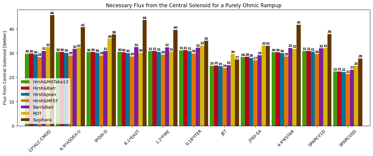
N.B that the poynting method is significantly lower than the Rule of Thumb (ROT) and the Sugihara method, because it explicitly takes into account the flux contribution from the vertical field created by the poloidal field coils.
Integrating the flux consumption algorithm with the rest of POPCON
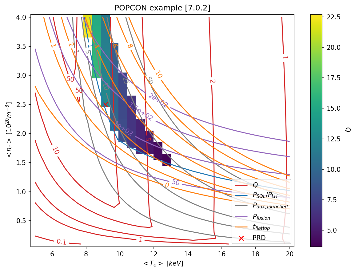
It is also of course possible to make a typical POPCON plot where the maximum flattop time can be seen in operation space. We’ve adapted the “SPARC_PRD” example to use the flux consumption algorithm. Therefore, running this calculation over a grid of values is as simple as the following.
[12]:
input_parameters, algorithm, points, plots  = cfspopcon.read_case("example_cases/SPARC_PRD")
algorithm.validate_inputs(input_parameters);

dataset = xr.Dataset(input_parameters)

dataset = algorithm.update_dataset(dataset)

plot_style = cfspopcon.read_plot_style("example_cases/SPARC_PRD/plot_popcon.yaml")

cfspopcon.plotting.make_plot(
    dataset,
    plot_style,
    points=points,
    title="POPCON example",
    output_dir=None
)